Advanced Data Visualizations
Comparing Objects
Comparing Objects Using the Image Object Table
To open this dialog select Image Objects > Image Object Table from the main menu.
This dialog allows you to compare image objects of selected classes when evaluating classifications. To launch the Configure Image Object Table dialog box, double-click in the window or right-click on the window and choose Configure Image Object Table.
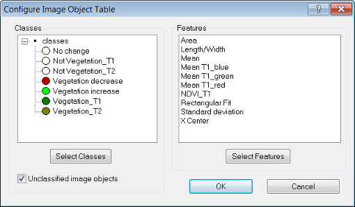
Upon opening, the classes and features windows are blank. Press the Select Classes button, which launches the Select Classes for List dialog box.
Add as many classes as you require by clicking on an individual class, or transferring the entire list with the All button. On the Configure Image Object Table dialog box, you can also add unclassified image objects by ticking the check box. In the same manner, you can add features by navigating via the Select Features button.
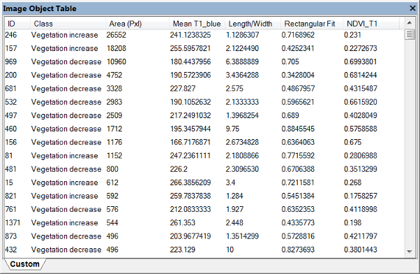
Clicking on a column header will sort rows according to column values. Depending on the export definition of the used analysis, there may be other tabs listing dedicated data. Selecting an object in the image or in the table will highlight the corresponding object.
In some cases an image analyst wants to assign specific annotations to single image objects manually, e.g. to mark objects to be reviewed by another operator. To add an annotation to an object right-click an item in the Image Object Table window and select Edit Object Annotation. The Edit Annotation dialog opens where you can insert a value for the selected object. Once you inserted the first annotation a new object variable is added to your project.
To display annotations in the Image Object Table window please select Configure Image Object Table again via right-click (see above) and add the Object feature > Variables > Annotation to the selected features.
Additionally, the feature Annotation can be found in the Feature View dialog > Object features > Variables > Annotation. Right-click this feature in the Feature View and select Display in Image Object Information to visualize the values in this dialog. Double-click the feature annotation in the Image Object Information dialog to open the Edit Annotation dialog where you can insert or edit its again.
Comparing Features Using the 2D Feature Space Plot
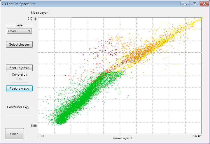
This feature allows you to analyze the correlation of two features of selected image objects. If two features correlate highly, you may wish to deselect one of them from the Image Object Information or Feature View windows. As with the Feature View window, not only spectral information maybe displayed, but all available features.
- To open 2D Feature Space Plot, go to Tools > 2D Feature Space Plot via the main menu
- The fields on the left-hand side allow you to select the levels and classes you wish to investigate and assign features to the x- and y-axes
The Correlation display shows the Pearson’s correlation coefficient between the values of the selected features and the selected image objects or classes.
Accuracy Assessment Tools
Accuracy assessment methods can produce statistical outputs to check the quality of the classification results. Tables from statistical assessments can be saved as .txt files, while graphical results can be exported in raster format.
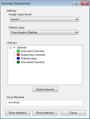
- Choose Tools > Accuracy Assessment on the menu bar to open the Accuracy Assessment dialog box
- A project can contain different classifications on different image object levels. Specify the image object level of interest by using the Image object level drop-down menu. In the Classes window, all classes and their inheritance structures are displayed.
- To select classes for assessment, click the Select Classes button and make a new selection in the Select Classes for Statistic dialog box. By default all available classes are selected. You can deselect classes through a double-click in the right frame.
- In the Statistic type drop-down list, select one of the following methods for accuracy assessment:
- Classification Stability
- Best Classification Result
- Error Matrix based on TTA Mask
- Error Matrix based on Samples
- To view the accuracy assessment results, click Show statistics. To export the statistical output, click Save statistics. You can enter a file name of your choice in the Save filename text field. The table is saved in comma-separated ASCII .txt format; the extension .txt is attached automatically.
Classification Stability
The Classification Stability dialog box displays a statistic type used for accuracy assessment.
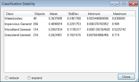
The difference between the best and the second best class assignment is calculated as a percentage. The statistical output displays basic statistical operations (number of image objects, mean, standard deviation, minimum value and maximum value) performed on the best-to-second values per class.
The Best Classification Result dialog box displays a statistic type used for accuracy assessment.
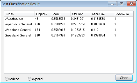
The statistical output for the best classification result is evaluated per class. To display the graphical output, go to the View Settings Window and select Mode > Best Classification Result. Basic statistical operations are performed on the best classification result of the image objects assigned to a class (number of image objects, mean, standard deviation, minimum value and maximum value).
Error Matrices
The Error Matrix Based on TTA Mask dialog box displays a statistic type used for accuracy assessment.
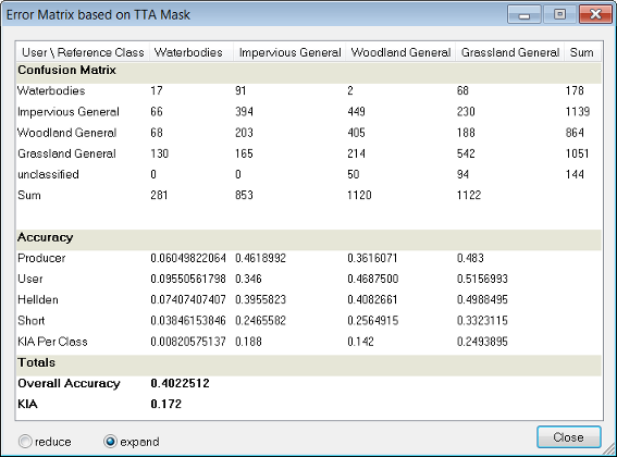
Test areas are used as a reference to check classification quality by comparing the classification with reference values (called ground truth in geographic and satellite imaging) based on pixels.
The Error Matrix Based on Samples dialog box displays a statistic type used for accuracy assessment.
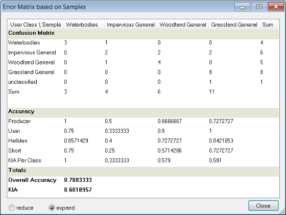
This is similar to Error Matrix Based on TTA Mask but considers samples (not pixels) derived from manual sample inputs. The match between the sample objects and the classification is expressed in terms of parts of class samples.
Polygons and Skeletons
Polygons are vector objects that provide more detailed information for characterization of image objects based on shape. They are also needed to visualize and export image object outlines. Skeletons, which describe the inner structure of a polygon, help to describe an object’s shape more accurately.
Polygon and skeleton features are used to define class descriptions or refine segmentations. They are particularly suited to studying objects with edges and corners.
A number of shape features based on polygons and skeletons are available. These features are used in the same way as other features. They are available in the feature tree under Object Features > Geometry > Based on Polygons or Object Features > Geometry > Based on Skeletons.
Polygon and skeleton features may be hidden – to display them, go to View > Customize and reset the View toolbar.
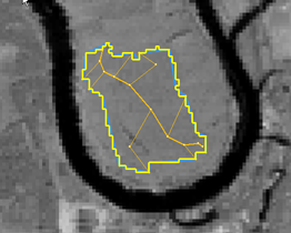
Viewing Polygons
Polygons are available after the first segmentation of a map. To display polygons in the map view, click the Show/Hide Polygons button (if activated deactivate Show or Hide outlines button first). For further options, open View > Display Mode > Edit Highlight Colors.
If the polygons cannot be clearly distinguished due to a low zoom value, they are automatically deactivated in the display. In that case, choose a higher zoom value.
Viewing Skeletons
Skeletons are automatically generated in conjunction with polygons. To display skeletons, click the Show/Hide Skeletons button and select an object. You can change the skeleton color in the Edit Highlight Colors settings.
To view skeletons of multiple objects, draw a polygon or rectangle, using the Manual Editing toolbar to select the desired objects and activate the skeleton view.
About Skeletons
Skeletons describe the inner structure of an object. By creating skeletons, the object’s shape can be described in a different way. To obtain skeletons, a Delaunay triangulation of the objects’ shape polygons is performed. The skeletons are then created by identifying the mid-points of the triangles and connecting them. To find skeleton branches, three types of triangles are created:
- End triangles (one-neighbor triangles) indicate end points of the skeleton A
- Connecting triangles (two-neighbor triangles) indicate a connection point B
- Branch triangles (three-neighbor triangles) indicate branch points of the skeleton C.
The main line of a skeleton is represented by the longest possible connection of branch points. Beginning with the main line, the connected lines then are ordered according to their types of connecting points.
The branch order is comparable to the stream order of a river network. Each branch obtains an appropriate order value; the main line always holds a value of 0 while the outmost branches have the highest values, depending on the objects’ complexity.
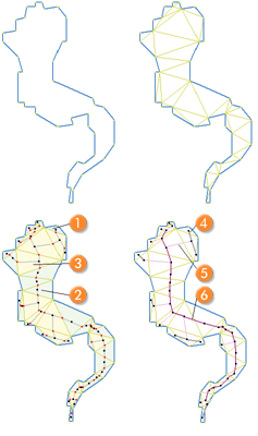
The right image shows a skeleton with the following branch order:
- 4: Branch order = 2.
- 5: Branch order = 1.
- 6: Branch order = 0 (main line).
